Elasticsearch - Grafana graphs

Grafana can pull from Elasticsearch as a data source, letting you build graphs and counters on top of your ELK stack logs. This post walks through the configuration from both sides: opening Elasticsearch for Grafana access, building queries in Kibana, and wiring it all up into Grafana panels.

Configure Elasticsearch

By default, network.host is set to 127.0.0.1 and commented out. Uncomment it and change the value to fit your environment. network.host accepts several formats. I want both Grafana and localhost to reach Elasticsearch:

network.host: 0.0.0.0

Then add or edit the two CORS lines:

http.cors.allow-origin: "*"
http.cors.enabled: true

Warning: Elasticsearch has no built-in security. Never bind it to an IP address reachable from servers you do not control. Do not bind it to a public or shared private network IP address.

Setting up the Grafana data source

Choose menu > Data sources > +Add new data source

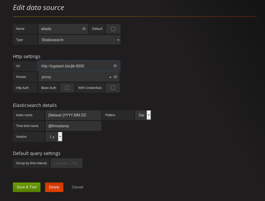
Give the data source a descriptive name so you can tell your sources apart. Set the type to Elasticsearch and fill in the URL to your Elasticsearch server. In this setup it is called logstash and access is set to proxy.

I use Filebeat to ship logs from servers to Logstash, which is why the index name follows that pattern. Elasticsearch stores data at the path set in path.data in elasticsearch.yml. Check that directory and you will see the index folder names — for example filebeat-2017-05-18. That is a folder, not a file.

The timefield name

Read the filter config in /etc/logstash/ to find the correct field name. I use a syslog filter with a custom timestamp field to make searching consistent:

filter {
  if [type] == 'syslog' {
    grok {
      match => { 'message' => '%{SYSLOGTIMESTAMP:syslog_timestamp} %{SYSLOGHOST:syslog_hostname} %{DATA:syslog_program}(?:\[%{POSINT:syslog_pid}\])?: %{GREEDYDATA:syslog_message}' }
      add_field => [ 'received_at', '%{@timestamp}' ]
      add_field => [ 'received_from', '%{host}' ]
    }
    syslog_pri { }
    date {
      match => [ 'syslog_timestamp', 'MMM d HH:mm:ss', 'MMM dd HH:mm:ss' ]
    }
  }
}

Now save and test. A green status means Grafana can reach Elasticsearch.

Kibana: build the search string

Log in to Kibana and open the Discovery pane. Kibana uses Lucene query syntax. For a syntax reference, see lucenetutorial.com.

The goal here is to count rejected mail on the MX servers. When a mail arrives, the MX server runs a postscreen check: a pregreeting check (did the sending server talk before it was allowed to?) and an RBL check against Spamhaus. The RBL check logs a rank of dnsbl 1 or dnsbl 2, so searching for dnsbl catches both.

This is a small excerpt from an MX server log. The search string *dnsbl returns two hits per log entry, which produces false positives when counting daily blocks.

Narrow it down by selecting specific search fields. In this case, filter on syslog_message.

The result shows the DNSBL hit count over any chosen time range. Save the search with a name that describes what it finds.

Open the visualization tool and choose the type that fits. A single-number counter gives a fast overview.

Pick “From a saved search” and select the search you saved. That is why naming matters.

The counter shows 16,347 hits in the last 15 minutes.

Graphs in Grafana

The setup mirrors what you did in Kibana.

Entries graph

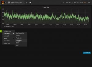
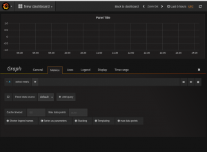
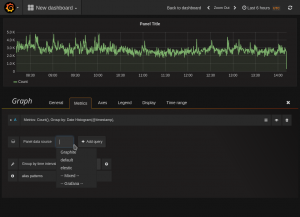
Add a graph panel to your dashboard. Click the green field on the right side of a row, choose “Add panel”, then “Graph”. Grafana selects the default data source — switch it to the Elasticsearch source you created. The graph populates with data. By default it uses a date histogram on @timestamp.

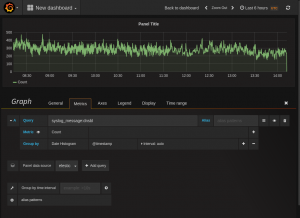
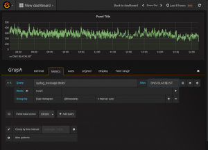
In the query field, enter the Lucene query string from Kibana, for example:

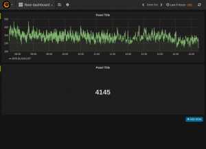
syslog_message:dnsbl

Grafana counts matching entries and plots them. Assign an alias to label the series. Return to the dashboard when done.

Singlestat panel

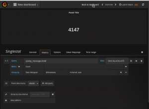
The procedure matches the graph setup. Singlestat panels support thresholds, alerting, and status coloring, which I will cover in a future post.